Defining Fire Return Intervals in Colorado for an Avoided Wildfire Emissions Protocol
The Modified Fire Return Interval map was developed to be used with the Avoided Wildfire Carbon Offset protocol by Anchor Point Group and CUSP. The materials are publicly available below in the “Materials Online” section. This information is provided “as is” without warrantee, but is the best information to date available for this purpose.
If you need guidence on how to use this map, or the Protocol itself, please contact Jeff Ravage or Jonathan Bruno at CUSP.
Materials Online
Coming Soon
Introduction
A greenhouse gas offset protocol centered on forest management practices intended to avoid or reduce emissions from wildfires developed for California (Greenhouse gas offset protocol: Avoided wildfire emissions in California; Version 10/18/2016) is being extended for application in Colorado. Methods outlined in the protocol are intended to quantify greenhouse gas offsets arising from fuel treatments that restore a forested area to desired ecological conditions and fire regimes.
A central component of the protocol’s methods is to estimate the fire return interval (FRI) for the vegetation community in a project area to assign a statistical fire probability over the period of time that a fuel treatment is expected to be useful. The California protocol uses unique map products which are not available for Colorado or other states. Here we outline a method that we believe will provide a valid FRI map for Colorado, and that may be extended to other states.
Justification of Data Set Choices
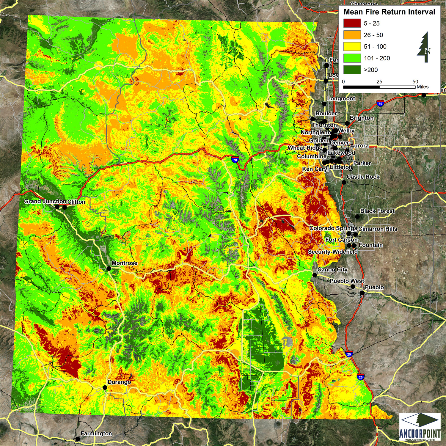
We start with the LANDFIRE (LF) Mean Fire Return Interval (MFRI; LANDFIRE 2014) map product as a baseline to provide general patterns in FRI based on both pre-Euro-American settlement fire regimes and vegetation structure. MFRI is derived from the vegetation and disturbance dynamics model, Vegetation Dynamics Development Tool (VDDT), and linked spatially using the LF Biophysical Settings (BpS) layer. BpS represents historical vegetation that likely was present prior to Euro-American settlement. A major component in defining BpS is the underlying physical and climatological environment of each individual pixel. These environmental factors constrain fuel productivity and fuel drying, the two factors that in turn affect fire occurrence. A conceptual foundation for these pyrogeographic processes is referred to as the varying constraints hypothesis (Krawchuk and Moritz 2011). Although LANDFIRE MFRI represents historical conditions, its underlying biophysical structure provides a peer-reviewed, nationally-seamless, ecological foundation with which to estimate current FRI for use in the Offset protocol.
We then modify MFRI by overlaying Burn Probability (BP) data developed from the Fire Simulation (FSim) modeling exercise (Finney et al 2011, Short et al. 2016). FSim simulates the occurrence and sizes of fires that burn under tens of thousands of potential fire years that are constrained by modern weather conditions, ignition likelihood, fire growth, and fire suppression activities. These multiple fire years are then summarized into a probability of a given pixel burning under current landscape conditions and fire management practices. Thus the combination of LANDFIRE MFRI coupled with FSim provides a summary of contemporary FRI to use in the Avoided Emissions Offset methods.
The LF MFRI map was chosen based on the data set’s concurrence with empirical studies on historic fire return intervals. However, LF MFRI methods reflect conditions more representative of pre-Euro-American settlement. To mitigate this limitation, FSim BP data were used because, while this approach used the same LANDFIRE inputs that MFRI is based on, BP uses weather and topography data (along with LF fuel/vegetation information) to simulate numerous wildfires and record the area burned. The aggregate of the perimeters of all simulated fires shows the pattern of fire susceptibility on the landscape. The combination of the LANDFIRE MFRI and FSim BP data sets was thought to be a stronger representation of mean fire return interval than either option by itself. As stated above, LF MFRI provides the ecological foundation which is then modified to current burning conditions using the BP layer.
The modified MFRI data set was further modified to reflect the role of people on the landscape in causing fires. Anchor Point’s National Hazard and Risk (No-HARM) data set contains a polygon data set representing the locations where people live and work. Polygons representing intermediate levels of human habitation were used to reduce the mean fire return interval values in areas within a specified distance of these community polygons.
Overview of MFRI Mapping Methods
- LF MFRI was used as the starting point for our fire return interval mapping effort.
- LF MFRI was partitioned by class and overlayed with FSim BP data to get a frequency distribution of BP data for each MFRI class
- Geographic areas representing the shorter side of the BP frequency distribution had their LF MFRI return interval values reduced
- The resulting MFRI layer was further modified using data from No-HARM intermediate density polygons.
- The above layer was then masked to only include the area in specific supersection polygons.
Peer Review Group
A peer review group was convened to discuss the approach, data utilization and future improvements for this task. The group consisted of senior staff and consultants representing federal, state and local expertise. Several group members were recently retired from agencies and therefore could not directly represent their previous employer, however their significant knowledge on fire-related issues was directly applicable to the review. Some of the participants were concerned that this protocol would drive project selection, this was then clarified. “It is not intended to be used as a tool to identify sites for treatment. In other words: our Fire Return Interval Map is a tool for modification of the final offset (avoided CO2 equivalent) not a tool for identification of project areas. The FRI map is just a small piece of the quantification equation – one that is unique to Colorado, but is not even the primary calculation of carbon storage/release. The main calculations for this protocol come from actual conditions on the project site – fuel load/type and conditions such as: weather patterns or the presence of insect or disease. As we may not have made clear, we are working towards a conservative estimate of Fire Return over large landscapes, project designers will be best served by running calculations on their project footprint at finer scales. As the project progresses we hope to have peer-reviewed modifications to FRI that will further enhance the calculated values. The choice of applying for carbon offset funding is not intended to be the primary method of funding or a mechanism of project administration”. With this clarification and after continued dialog on the approach and methodology the group offered full support and agreement with the current approach.
Peer Review Group Participants
Mike Babler, Teocalli Consulting (formerly with the Colorado State Forest Service and the Nature Conservancy)
Peter Brown, Rocky Mountain Tree-Ring Research
Tony Cheng, Colorado State University (Dept. of Forest and Rangeland Stewardship, Director of the Colorado Forest Restoration Institute)
Jonathan Bruno, Coalition for the Upper South Platte
Boyd Lebeda, District Forester, Colorado State Forest Service
Mark McLean, Anchor Point
Jeff Ravage, Coalition for the Upper South Platte
Todd Ricardson, Bureau of Land Management/CO Fire Management Officer (Type II Incident Commander)
Mike Smith, RenewWest
Ross Willmore, Wildfire Management Solutions (formerly East Zone Fire Management Officer, Eagle, CO)
Chris White, Anchor Point
Establishing Area of Interest
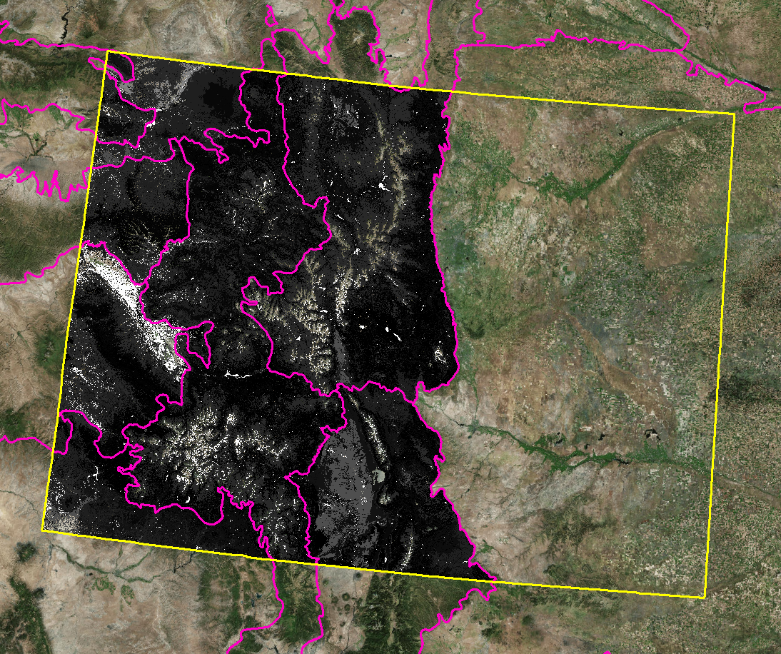
Following discussion with the peer review group, the data were also clipped to focus on areas primarily consisting of shrub and timber. This was done using “supersections,” from the Climate Action Reserve’s Forest Project Protocol.[1] The polygons covering the western portion of the State were chosen as the project Area of Interest (AOI) (Figure 1).
LANDFIRE MFRI Modification using FSim Burn Probability
As stated above, our method started with the LF MFRI data set. In its raw form, LF MFRI, consists of a series of increasingly-wide classes of years of return interval (Table 1).
| LF Value | Return Interval Range (Years)/Description | Converted Value |
| 1* | 0-5 | 3 |
| 2 | 6-10 | 8 |
| 3* | 11-15 | 13 |
| 4 | 16-20 | 18 |
| 5 | 21-25 | 23 |
| 6 | 26-30 | 28 |
| 7 | 31-35 | 33 |
| 8 | 36-40 | 38 |
| 9* | 41-45 | 43 |
| 10 | 45-50 | 48 |
| 11 | 51-60 | 55 |
| 12 | 61-70 | 65 |
| 13 | 71-80 | 75 |
| 14* | 81-90 | 85 |
| 15* | 91-100 | 95 |
| 16 | 101-125 | 113 |
| 17 | 126-150 | 138 |
| 18 | 151-200 | 175 |
| 19* | 201-300 | 250 |
| 20* | 301-500 | 400 |
| 21* | 501-1000 | 750 |
| 111 | Water | N/A |
| 112 | Snow/Ice | N/A |
| 131 | Barren | N/A |
| 132 | Sparsely Vegetated | N/A |
| 133 | Indeterminate Fire Regime | N/A |
Table 1: LANDFIRE MFRI Values, Year Ranges and Converted Values. Asterisks in the first column indicate classes that were not adjusted by BP values either due to zero values for the 1st quartile or due to extremely low pixel counts.
The values in the left column are those that appear in the raw LF MFRI data. The middle column of data is the description of the values. Continued analysis of the MFRI data necessitated the conversion from descriptive values to the year equivalent of each value. Since the values for the first 21 entries in the table represent ranges of years, the median value (rounded up to the nearest integer) was chosen as the single value (in years) that best represents the range of years. Raw values greater than 21 were omitted from the data set since they do not have years associated with them. The result of the conversion of the raw values to their year equivalents was a spatial raster covering Colorado with a return interval (in years) for each pixel (or a NoData value for those pixels with raw values greater than 21).
The resulting modified LF MFRI data set was then compared to 15 field study sites to assess their correspondence with empirical data. The sites are where tree-ring fire history studies have been developed in central Colorado (Brown and Shepperd 2001). We compared the published MFRI results with the LF MFRI map layer.There was relatively broad agreement between LF MFRI and field data, although in general not at individual 30m point locations. Field site locations were presented as single point data even though samples were collected from polygons around the point. To better capture the general locational MFRI, we decided to use a moving window mean analysis to smooth the data set. A 270m window size was decided on after visual analysis of the data set relative to aerial photography and because this matches the raw pixel size of the FSim BP data set. The resulting data set was LF MFRI (modified from raw values to years representing the associated ranges) smoothed with a 270m moving window analysis that calculated the mean for the pixel at the center of the window.
This post-moving window analysis, modified LF MFRI data set was then further adjusted due to the fact that LF MFRI 1) is primarily representative of pre-Euro-settlement conditions and 2) paints much of the landscape with similar values, regardless of current conditions such as time since previous disturbance. The post-moving window analysis data set still contains the patterns imposed due to these data limitations. FSim BP was used to further adjust the modified LF MFRI by the inclusion of relatively-local weather conditions and topographic influence on fire burn patterns. This adjustment was accomplished by overlaying each of the return interval classes independently with spatially co-occurring values of FSim BP. A separate frequency distribution of FSim BP values was calculated for each LF MFRI return interval value. The first quartile was calculated for each of the frequency distributions and and any values pixels that contained an FSim BP value below the 1st quartile value were identified for having their modified LF MFRI value reduced. The only exceptions to the above were that a class was not identified for reduction if the 1st quartile was calculated to be zero or if the pixel count of the class was very small (these classes are marked with an asterisk in Table 1).
At this point in the analysis, pixels have been identified to have their return interval values reduced, but the amount of reduction had not yet been decided. We decided on a single reduction factor due to a perceived lack of meaningful granularity in the FSim BP data set. The single value of reduction was selected by analyzing the means and standard deviations from the 15 field studies mentioned previously. By looking at the ratio of the means and standard deviations across the 15 field sites, a reduction value of 25% was selected. Therefore, the pixels marked for reduction in the previous step were multiplied by 0.75 to reduce their return interval values.
Inclusion of Intermix and Interface Data as MFRI Reduction Factor
Proximity to areas of human habitation has been identified as an element that could alter mean fire return intervals and this idea was supported by the Peer Review Group. It has been noted that the relationship between human activity and fire frequency may not be linear, with higher levels of human activity reducing fire frequency and intermediate levels increasing activity[1],[2] (Syphard et al. 2007; Parisien et al. 2012). One potential explanation for this pattern is that higher “levels of activity” (or human habitation density) is that all areas of human habitation come with additional risk for wildfire ignition in the form of children playing with matches, cigarette-smoking, heavy machinery use, etc.. However, in higher-density areas, these risks can be mitigated by additional suppression resources. Medium-density areas are less likely to have such resources and lower-density areas have reduced risk and suppression resources (potentially “cancelling out” added risk and lack of suppression resources).
Justification of the Use of No-HARM’s Interface/Intermix Layers
Because it was thought that return intervals were already representative of the upper portions of the range of historic variability in the LF MFRI data set, we decided not to apply an increase in return interval values in areas adjacent to the highest densities of human habitation. To capture the pattern of increased fire frequency in areas adjacent to intermediate levels of human activity, however, we decided to use a data set that has already identified intermediate levels of human habitation. To make a spatial adjustment to the modified LF MFRI data set, we used an existing intermediate map of housing density used as input information to produce Anchor Point’s National Hazard and Risk Model (No-HARM) data set (used to assess and map wildfire risk nation-wide). One of the intermediate products that improves the accuracy of No-HARM is the identification of where people live at two different housing densities. The highest density level represents the edges of cities and towns where typical urban and suburban neighborhoods meet wildland fuel areas (this density level was not used). Intermix structure density is representative of intermediate housing densities where wildland fuel may be present between houses and throughout the neighborhood but where suppression resources are limited in comparison to the edges of cities and towns. Both housing density thresholds were mapped using parcel centroids and US Postal Service Zip + 4 information. To streamline nomenclature, we will refer to the intermix and interface polygons as simply Wildland Urban Interface or “WUI.”
Buffer Analysis Description
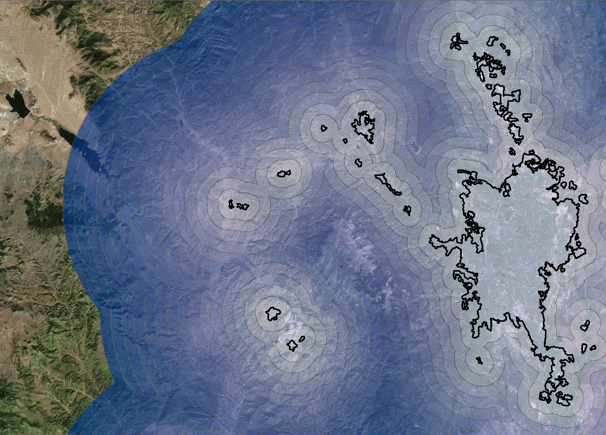
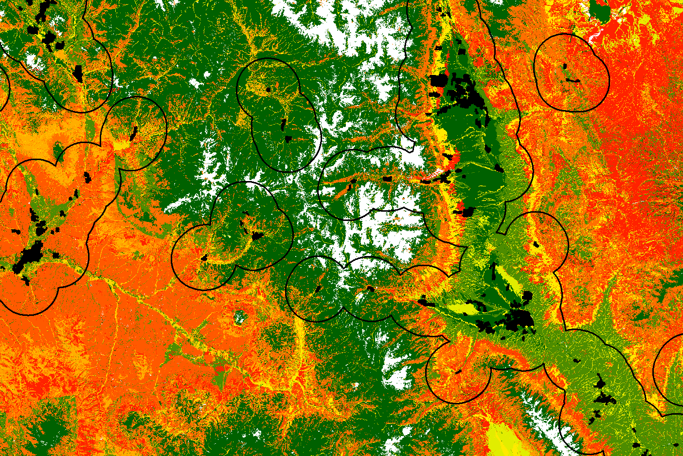
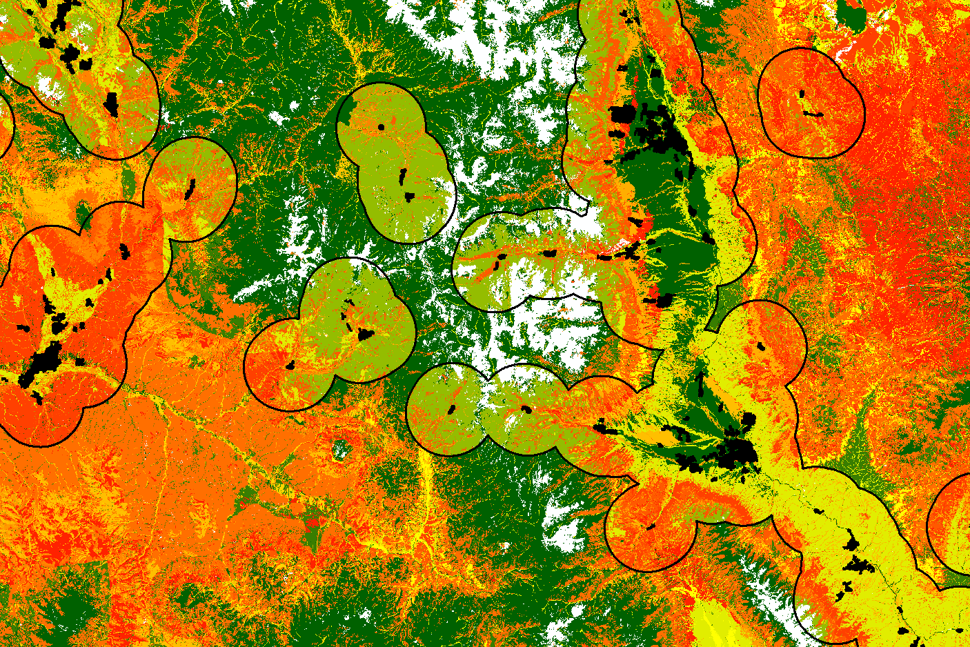
To determine the method for using the WUI polygon map, some exploratory data analysis was conducted. We needed to decide on a distance from WUI polygons that a reduction would take place and the amount of reduction needed to be decided. To aid in making these decisions, we decided to use buffers to analyze the trend of wildfire frequency and acres burned as distance from WUI polygons increased. 15 buffers in 1-mile increments were generated for WUI polygons (Figure 2) which were used in subsequent steps of the analysis.
Comparison of Buffers with Ignition Points
The buffers were used to examine distance decay patterns away from WUI polygons vs. a fire ignition point data set. The Fire Program Analysis (FPA) system[1] has produced an exhaustive data set identifying the location (points) of human-caused (anthropogenic) and natural fire ignitions from 1992 to 2015. Human-caused fires in this data set would be assumed to be spatially collinear with No-HARM’s WUI data if the patterns discussed (intermediate human activity levels vs. fire frequency) are relevant in Colorado. To assess the spatial similarity of the data sets, the 15 1-mile buffers around WUI polygons were used to select any anthropogenic ignition points that occurred within their boundaries, the densities of anthropogenic ignitions in each buffer were calculated, and the results were graphed in Figure 3.
The pattern in the graph does support the hypothesis that human activity (represented by WUI polygons) has an impact on human-caused ignitions. The highest density of human-caused ignitions occurs within 1-mile of WUI polygons. The density of ignitions decreases quickly with distance, however. The gray line represents the background density of human-caused ignitions across all of Colorado. Human-caused ignition density is lower than the background density beyond 3 miles away from intermix and interface polygons. The pattern in this graph (and in Figure 5) was thought by the peer review group to be adequate justification for the use of No-HARM WUI polygons.
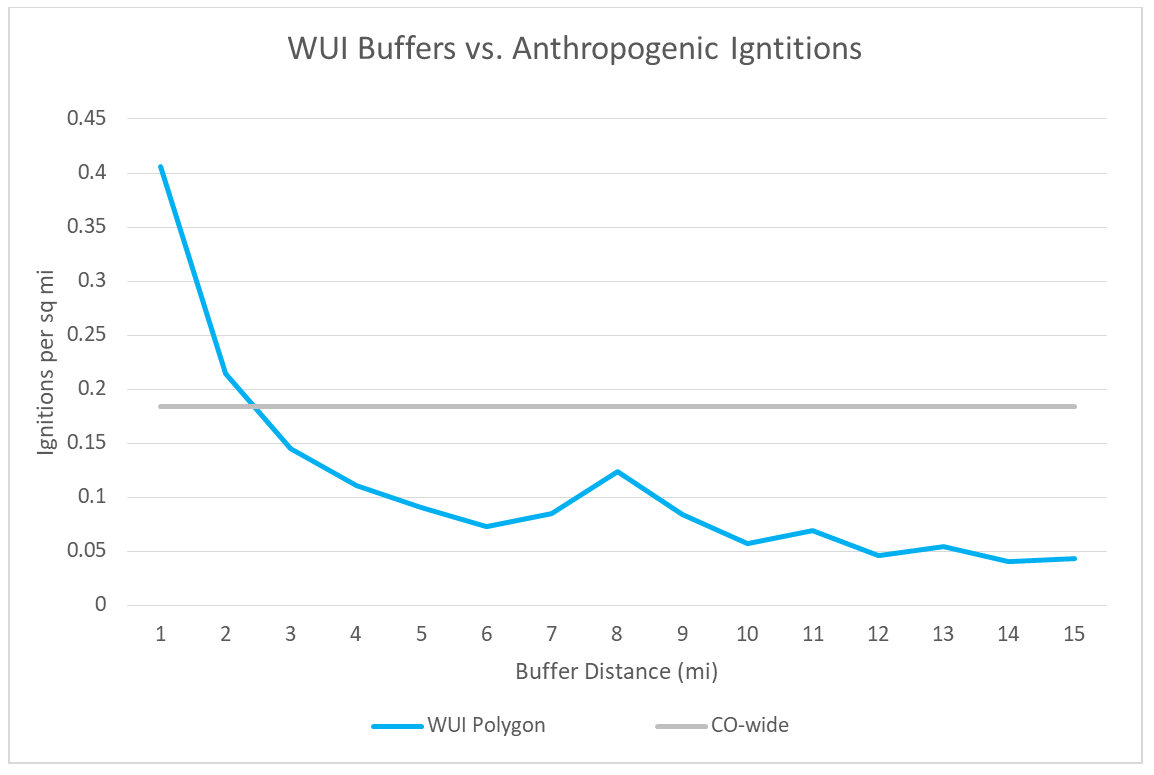
Figure 3: WUI Polygon buffers vs. anthropogenic ignition density
Comparison of Buffers with Fire Perimeters (Burned Areas)
The use of the ignition data set for comparison with WUI areas was appropriate because of the obvious causal link between the two data sets (fires caused by people should occur where people spend most of their time). However, ignitions do not cause changes to carbon sequestration in and of themselves – they must become wildfires before this happens. A data set showing where conversion of carbon in the form of historic fire has occurred would be more appropriate for determining where and how much to alter the modified LF MFRI map. There are many such data sets, but the Geospatial Multi-Agency Coordination (GeoMAC)[1] wildfire perimeter data set has nation-wide coverage and is standardized from state to state. GeoMAC has polygon data for wildfire perimeters that occurred between 2000 and 2016 (GeoMAC has perimeters for fires up to the present day, but we decided to stop our analysis at 2016).
This data set was used with the WUI polygon buffers created previously to determine how much area was burned in concentric 1-mile buffers away from interface and intermix (WUI communities). The data were first converted from vector (polygons) to raster format. This then allowed zonal statistics (summation of all burned cells) within each buffer zone. The total area of each buffer zone was then used to convert the summed burned area to a percentage of area burned. Figure 3 shows the resulting graph.
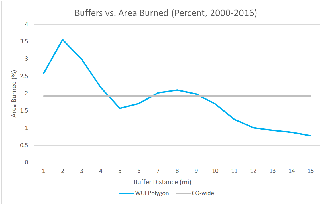
Figure 4: WUI polygon bBuffers vs. percentage of buffer area burned
Unlike the previous results (Figure 2), the shape of the curve for WUI polygon buffers was different. The buffers around WUI polygons, especially the first 3 miles of buffers than farther buffers. which are much higher than the line representing the background percentage burned for Colorado (gray line). At four years and beyond, the percentage burned value dips below the average for the rest of the area of Colorado. Therefore, we decided to use the 3-mile buffer around intermix polygons as the spatial extent of our further adjustments to the MFRI.
Reduction of MFRI Within 3 Miles of WUI Polygons
The final element of the spatial adjustment of the modified MFRI map within 3 miles of WUI polygons is the magnitude of the adjustment. We determined this value by averaging the departures (as a ratio) between the percent burned area in each of the three closest buffer areas (miles 1 to 3) and the Colorado-wide percentage burned values. These three numbers were .75, .54 and .64. The average of these three numbers is 0.64. It is this average departure value (from Colorado-wide burned percentages) that we used as an adjustment value for the MFRI map.
Conclusion and Next Steps
The modified MFRI map is an adequate start for use in the Avoided Wildfire Emissions Protocol. It provides an excellent baseline that can be easily augmented in later phases of the project.
To make the data set better at forecasting conditions into the future, climate change modeling would need to be used and incorporated into the modified LF MFRI data set. The existing data set could again be used as a baseline for inclusion of climate forecasts, but these adjustment factors should be used so that a more accurate representation of project lifetimes can be made.
[1] http://www.climateactionreserve.org/how/protocols/forest/assessment-area-data/ Accessed 6/20/2017
[2] Syphard, AD, VC Radeloff, JE Keeley, TJ Hawbaker, MK Clayton, SI Steward and RB Hammer (2007) Human influence on California fire regimes. Ecological Applications 17(5):1388-402.
[3] Parisien, MA, S Snetsinger, JA Greenberg, CR Nelson, T Schoennagel, SZ Dobrowski and MA Moritz. (2012) Spatial variability in wildfire probability across the western United States. International Journal of Wildland Fire 21:313-327.
[4] Short, Karen C. 2017. Spatial wildfire occurrence data for the United States, 1992-2015 [FPA_FOD_20170508]. 4th Edition. Fort Collins, CO: Forest Service Research Data Archive. https://doi.org/10.2737/RDS-2013-0009.4
[5] https://www.geomac.gov/
References
https://www.geomac.gov/
Brown, P.M., and W.D. Shepperd. 2001. Fire history and fire climatology along a 5° gradient in latitude in Colorado and Wyoming, USA. Palaeobotanist 50:133-140.
Krawchuk, MA, and MA Moritz (2011) Constraints on global fire activity vary across a resource gradient. Ecology 92:121-132.
LANDFIRE 2014 (LF .14.0), Mean Fire Return Interval Layer, LANDFIRE 1.4.0, U.S. Department of the Interior, Geological Survey. Accessed 5 May 2017 at
http://landfire.cr.usgs.gov/viewer/
Parisien, MA, S Snetsinger, JA Greenberg, CR Nelson, T Schoennagel, SZ Dobrowski and MA Moritz. (2012) Spatial variability in wildfire probability across the western United States. International Journal of Wildland Fire 21:313-327.
Short, Karen C.; Finney, Mark A.; Scott, Joe H.; Gilbertson-Day, Julie W.; Grenfell, Isaac C. 2016. Spatial dataset of probabilistic wildfire risk components for the conterminous United States. Fort Collins, CO: Forest Service Research Data Archive. https://doi.org/10.2737/RDS-2016-0034
Syphard, AD, VC Radeloff, JE Keeley, TJ Hawbaker, MK Clayton, SI Steward and RB Hammer (2007) Human influence on California fire regimes. Ecological Applications 17(5):1388-402.